어텐션과 로짓 들여다보기

이 챕터에서 배우는 것

• head 별 attention map 시각화 — 모델이 무엇을 보고 있나
• top-k logit 추적 — 다음 토큰 후보 분포의 모양
• 학습 전 / 후 비교 — 학습이 어떻게 attention 을 형성하나
• 실패 사례 디버깅 워크플로우 — 모델이 깨지는 자리

전제

Ch 8 Attention, Ch 10 nanoGPT. 학습된 모델 (Ch 15 의 final.pt) 가 손에 있어야 함.

---

1. 개념 — 모델 내부의 두 가지 신호

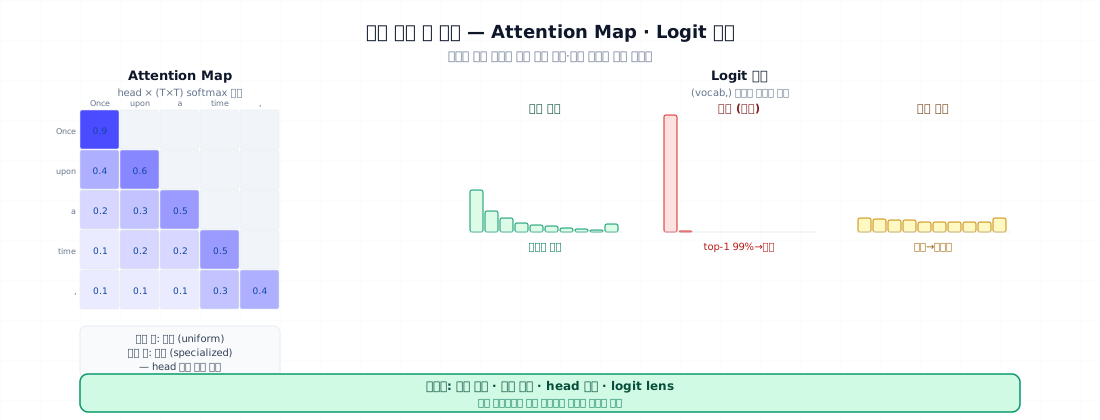
PPL · 벤치마크 · 사람 평가 모두 모델 출력 을 본다. 한 단계 안으로 들어가면:

신호	무엇	무엇을 답함
Attention map	각 head 의 (T, T) softmax 행렬	"토큰 i 가 j 를 얼마나 보나"
Logit 분포	마지막 layer 의 (vocab,)	"다음 토큰 후보들의 확신도"

이 둘이 모델이 무엇을 학습했는가 의 직접적 증거. 디버깅·연구·신뢰성에 모두 필요.

---

2. 왜 들여다보나

학습 진단

학습 전후 attention map 비교 → head 가 어떤 패턴을 학습했나 확인.

• 학습 전: 균등 (uniform) — 모든 위치 비슷한 가중치
• 학습 후: specialization — head 마다 다른 패턴 (직전 토큰 / 첫 토큰 / 마지막 명사 등)

실패 사례 분석

생성 결과가 이상할 때 (예: 같은 단어 반복) — logit 분포 보면 즉시 진단:

• 분포가 한 토큰에 99% — temperature 너무 낮거나 모델이 깨짐
• 분포가 평평 (top-1 1%) — 모델이 헷갈림, 학습 부족 신호

신뢰성 검증

PPL 좋은데 출력 이상 → 내부가 어떻게 작동하는지. 본 책 10M 동화 모델 같은 작은 모델일수록 직접 보는 게 유일한 디버깅 도구.

---

3. 어디에 쓰이나 — 5가지 표준 패턴

큰 모델 분석에서 발견된 head 의 전형적 학습 패턴:

패턴	무엇을 보나	어디
Previous token	직전 토큰	모든 layer
First token (BOS)	시퀀스 시작	깊은 layer
Diagonal (self)	자기 자신	모든 layer
Induction	같은 문맥 이전 위치	중간 layer (Anthropic 발견)
Position-skip	일정 거리 떨어진 위치	표제어·반복 패턴

본 책 10M 모델은 layer 6, head 8 = 48 head. 그중 1~2 개가 induction 비슷한 패턴 학습할 가능성. 작은 모델이라 명확히 안 잡힐 수도.

---

4. 최소 예제 — Attention map 추출

F.scaled_dot_product_attention 은 attention 가중치를 반환 안 함 (FlashAttention 메모리 최적화). 시각화 위해 수동 구현으로 한 번 더 forward.

import torch
import torch.nn.functional as F
from nano_gpt import GPTMini, GPTConfig, apply_rope
import matplotlib.pyplot as plt

cfg = GPTConfig(...)
model = GPTMini(cfg).cuda().eval()
state = torch.load("runs/exp1/final.pt")
model.load_state_dict(state['model'])

@torch.no_grad()
def get_attention(model, x):
    """모든 layer 의 (head, T, T) attention map 반환."""
    cos, sin = model.cos, model.sin
    h = model.tok_emb(x)
    maps = []
    for block in model.blocks:
        # block.attn 의 forward 를 수동 재현                           (1)
        attn = block.attn
        B, T, D = h.shape
        normed = block.norm1(h)
        q, k, v = attn.qkv(normed).split(D, dim=-1)
        q = q.view(B, T, attn.n_head, attn.head_dim).transpose(1, 2)
        k = k.view(B, T, attn.n_head, attn.head_dim).transpose(1, 2)
        v = v.view(B, T, attn.n_head, attn.head_dim).transpose(1, 2)
        q = apply_rope(q, cos[:T], sin[:T])
        k = apply_rope(k, cos[:T], sin[:T])

        scores = (q @ k.transpose(-2, -1)) / (attn.head_dim ** 0.5)
        mask = torch.triu(torch.ones(T, T, device=x.device), 1).bool()
        scores = scores.masked_fill(mask, float('-inf'))
        att = F.softmax(scores, dim=-1)                                 # (2)
        maps.append(att[0].cpu())                                       # (head, T, T)

        # 원래 forward 진행
        out = att @ v
        out = out.transpose(1, 2).contiguous().view(B, T, D)
        h = h + attn.proj(out)
        h = h + block.ffn(block.norm2(h))
    return maps                                                         # list of (head, T, T)

# 사용
text = "Once upon a time, there was a little girl named"
ids = torch.tensor([tok.encode(text).ids], device='cuda')
maps = get_attention(model, ids)
print(f"  layers: {len(maps)}, heads: {maps[0].shape[0]}")

1. SDPA 내부를 직접 풀어 attention 가중치 (att) 를 추출.
2. softmax 결과가 attention map.

시각화

def plot_attention(maps, tokens, layer=0, head=0):
    att = maps[layer][head].numpy()
    fig, ax = plt.subplots(figsize=(8, 8))
    im = ax.imshow(att, cmap='Blues', aspect='auto')
    ax.set_xticks(range(len(tokens))); ax.set_xticklabels(tokens, rotation=45)
    ax.set_yticks(range(len(tokens))); ax.set_yticklabels(tokens)
    ax.set_xlabel("attended to"); ax.set_ylabel("from position")
    ax.set_title(f"Layer {layer}, Head {head}")
    plt.colorbar(im); plt.tight_layout(); plt.show()

tokens = [tok.decode([i]) for i in ids[0].tolist()]
plot_attention(maps, tokens, layer=2, head=3)

본 책 모델 (학습 후) 에서 자주 보이는 패턴:

• layer 0~1: 거의 자기 자신 또는 직전 (학습 안 된 head 도 다수)
• layer 2~3: 일부 head 가 첫 토큰 (BOS) 에 가중
• layer 4~5: 마지막 명사 (예: "girl") 에 attention 집중 — induction 시작

---

5. 실전 — Logit 분포 추적

@torch.no_grad()
def top_k_trace(model, tok, prompt, n_steps=10, k=5):
    """다음 n 토큰 생성하면서 매 step 의 top-k 후보 출력."""
    ids = torch.tensor([tok.encode(prompt).ids], device='cuda')
    for step in range(n_steps):
        logits, _ = model(ids)
        probs = F.softmax(logits[0, -1], dim=-1)
        top = torch.topk(probs, k)

        print(f"\nstep {step}: prefix='{tok.decode(ids[0].tolist())}'")
        for p, i in zip(top.values.tolist(), top.indices.tolist()):
            print(f"    {tok.decode([i]):>15s}  {p:.4f}")

        # greedy 로 다음 토큰
        ids = torch.cat([ids, top.indices[:1].unsqueeze(0)], dim=1)

top_k_trace(model, tok, "Once upon a time", n_steps=8, k=5)

전형적 출력 (본 책 모델):

step 0: prefix='Once upon a time'
    ,             0.6234
    ,Ġthere       0.1521
    Ġin           0.0432
    Ġthere        0.0398
    ĠLily         0.0287

step 1: prefix='Once upon a time,'
    Ġthere        0.7821         <-- 거의 확정
    ĠLily         0.0934
    Ġin           0.0421
    ...

관찰 가이드:

• Top-1 확률이 매우 높음 (>0.7): 모델이 다음 토큰 확신. 정형 표현 ("Once upon a time, there").
• Top-5 가 비슷한 확률: 모델이 헷갈림. 인명·명사 자리에서 흔함.
• Top-1 < 0.1: 모델이 모름. 학습 부족 또는 OOD.

---

6. 학습 전·후 비교

학습 안 된 모델 (random init) 과 학습 후 비교:

# 학습 전
model_init = GPTMini(cfg).cuda().eval()
maps_before = get_attention(model_init, ids)

# 학습 후
model_trained = GPTMini(cfg).cuda().eval()
model_trained.load_state_dict(torch.load("runs/exp1/final.pt")['model'])
maps_after = get_attention(model_trained, ids)

# Layer 2, head 3 비교
fig, (ax1, ax2) = plt.subplots(1, 2, figsize=(14, 6))
ax1.imshow(maps_before[2][3], cmap='Blues')
ax1.set_title("학습 전 (random init)")
ax2.imshow(maps_after[2][3], cmap='Blues')
ax2.set_title("학습 후 (12K step)")
plt.show()

예상 결과:

• 학습 전: 거의 균등 (uniform) — 마스크된 부분 빼고 모두 비슷한 색
• 학습 후: 대각선 + 첫 토큰 (BOS) + 일부 명사 에 집중

이게 학습이 attention 을 형성한 증거. 모델 능력의 직접적 시각화.

---

7. 자주 깨지는 포인트

1. SDPA 의 attention 가중치 추출 시도 — is_causal=True 면 가중치 반환 안 함. 수동 구현 필수.

2. 모든 layer × 모든 head 출력 — 6 × 8 = 48 plot. 너무 많음. layer 0/3/5, head 0/3/7 같은 샘플링.

3. attention map 의 색깔 절대값 비교 — 시각화는 normalize 함. 다른 plot 끼리 색 비교 불가. scale 명시.

4. logit 출력에 BPE 토큰 그대로 — Ġ, Ġthe 같은 표시가 헷갈림. tok.decode 한 번.

5. softmax 후 logit 비교 — softmax 는 monotonic 이지만 모양이 변함. 분포 비교는 logit 자체 또는 entropy 같이.

6. KV cache 모드에서 attention 추출 시도 — KV cache 가 들어가면 attention shape 가 다름. 분석은 cache 없이.

7. random init 과 비교 안 함 — "이 head 가 직전 토큰을 본다" 가 학습 효과인지 random 인지 모름. 항상 베이스라인 비교.

---

8. 운영 시 체크할 점

분석 워크플로우:

• 학습 전 (random init) 모델 메모리에 보관
• 학습 후 모델 로드
• 같은 prompt 로 두 모델 attention 추출
• layer × head 그리드 (예: 3×3 샘플) plot
• 학습 후 specialization 패턴 식별 (직전 / BOS / induction)
• logit top-5 trace 로 생성 흐름 확인
• 실패 사례 (반복·환각) 의 logit 분포 분석
• 분석 결과를 모델 카드 (Ch 22) 의 "한계" 섹션에 반영

---

9. 연습문제

1. 본 책 10M 모델로 §4 의 attention 추출. layer 0, layer 5 의 head 들 중 가장 sparse 한 (한 곳에 집중) head 를 찾아라.
2. 학습 step 1K, 5K, 12K 의 체크포인트로 같은 prompt 의 attention 을 비교. 학습 진행에 따라 어떻게 변하나?
3. §5 의 logit trace 를 temperature 0.0 (greedy) vs 0.8 로 같은 prompt 에 적용. top-1 확률이 어떻게 변화하는가?
4. 본 책 모델이 잘못 생성한 문장 (예: 갑작스런 화제 전환) 을 찾아 그 자리의 attention 을 분석. 어느 head 가 잘못된 자리를 보았나?
5. (생각해볼 것) induction head (Anthropic 발견) 가 본 책 10M 모델에서 형성되는가? 어떻게 검증할 수 있나?

---

Part 5 마무리

챕터	무엇을
Ch 16	PPL — 식·한계·생성 검토 프로토콜
Ch 17	HellaSwag-tiny · 도메인 probe · pass@k · LLM judge
Ch 18	attention map · logit 분포 — 모델 내부 신호

다음 단계 → Part 6 추론·배포. 학습된 모델을 양자화하고 띄우는 차례.

---

원전

• Vig (2019). A Multiscale Visualization of Attention in the Transformer Model. arXiv:1906.05714
• Elhage et al. / Anthropic (2021). A Mathematical Framework for Transformer Circuits. — induction head 개념
• Olsson et al. / Anthropic (2022). In-context Learning and Induction Heads. arXiv:2209.11895
• Karpathy. nanoGPT 의 attention 시각화 노트북