Peeking at Attention and Logits¶

What you'll learn
- Per-head attention map visualization — what the model is actually looking at
- Top-k logit tracing — the shape of the next-token probability distribution
- Before vs after training comparison — how training forms attention patterns
- Debugging workflow for failure cases — where the model breaks
Prerequisites
Ch 8 Attention, Ch 10 nanoGPT. You need the trained model from Ch 15 (final.pt) in hand.
1. Two signals inside the model¶
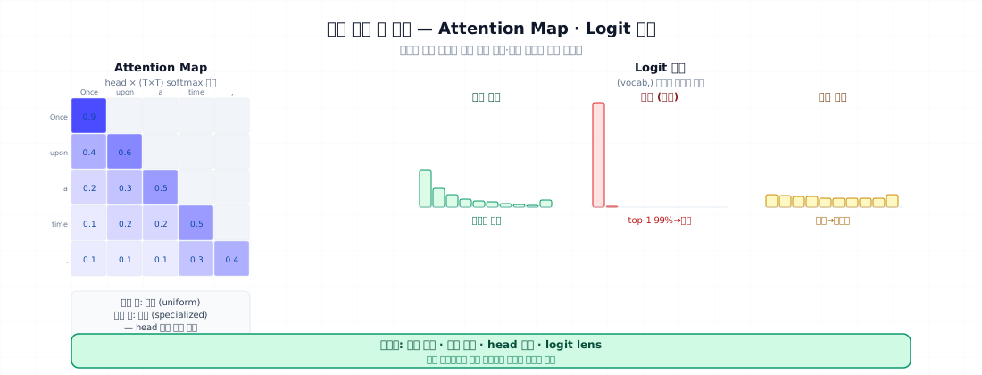
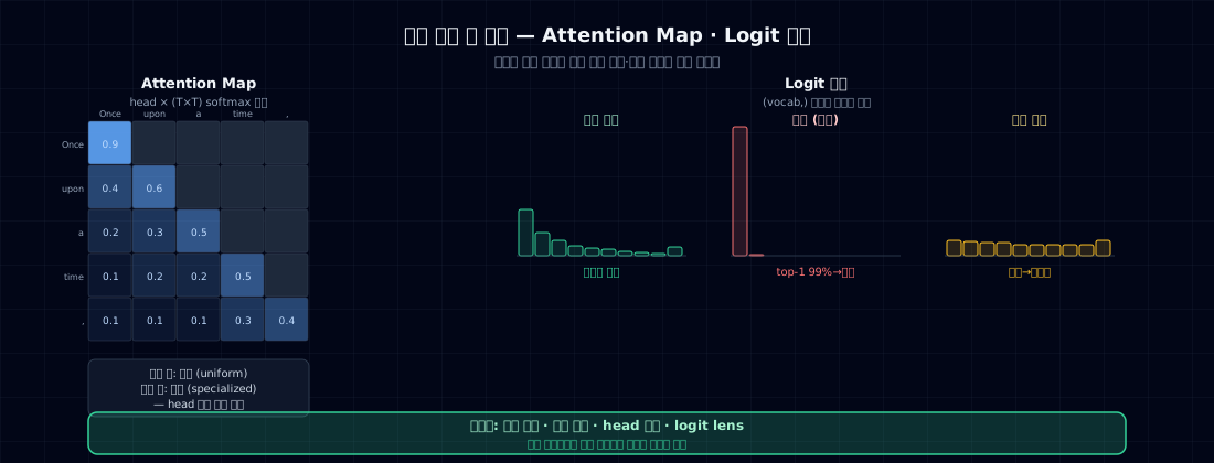
PPL, benchmarks, and human evaluation all look at model outputs. One level deeper:
| Signal | What it is | What it answers |
|---|---|---|
| Attention map | (T, T) softmax matrix per head | "how much does token i look at j?" |
| Logit distribution | (vocab,) from the final layer | "confidence over next-token candidates" |
These two are direct evidence of what the model has learned. Both are needed for debugging, research, and reliability work.
2. Why look inside¶
Training diagnostics¶
Comparing attention maps before and after training → confirms which patterns each head learned.
- Before training: uniform — similar weights across all positions
- After training: specialization — each head develops a different pattern (previous token / first token / last noun / etc.)
Failure case analysis¶
When generation goes wrong (e.g., repeating the same word) — look at the logit distribution for an immediate diagnosis:
- Distribution concentrated at one token (99%) — temperature too low or model is broken
- Flat distribution (top-1 at 1%) — model is confused, insufficient training signal
Reliability verification¶
Good PPL but strange output → what's happening inside? For small models like this book's 10M model, looking directly is often the only debugging tool.
3. 5 standard attention patterns¶
Patterns commonly found in large model analysis:
| Pattern | What it attends to | Where |
|---|---|---|
| Previous token | the immediately preceding token | all layers |
| First token (BOS) | start of sequence | deeper layers |
| Diagonal (self) | the token itself | all layers |
| Induction | earlier positions with matching context | middle layers (discovered by Anthropic) |
| Position-skip | a fixed distance away | headings, repetition patterns |
This book's 10M model has 6 layers × 8 heads = 48 heads. One or two of them may develop something resembling induction. With such a small model, the pattern might not be clear-cut.
4. Minimal example — extracting attention maps¶
F.scaled_dot_product_attention doesn't return attention weights (FlashAttention memory optimization). To visualize them, you need to manually reimplement the forward pass.
- Unrolling SDPA internals manually to extract the attention weights (
att). - The softmax output is the attention map.
Visualization¶
Patterns commonly visible in this book's trained model:
- Layers 0~1: mostly self or previous token (some heads still unspecialized)
- Layers 2~3: some heads weighted toward the first token (BOS)
- Layers 4~5: attention concentrating on the last noun (e.g., "girl") — early induction
5. Tracing the logit distribution¶
Typical output (this book's model):
step 0: prefix='Once upon a time'
    ,             0.6234
    ,Ġthere       0.1521
    Ġin           0.0432
    Ġthere        0.0398
    ĠLily         0.0287

step 1: prefix='Once upon a time,'
    Ġthere        0.7821         <-- almost certain
    ĠLily         0.0934
    Ġin           0.0421
    ...
Reading guide:
- Top-1 probability very high (>0.7): the model is confident about the next token. Formulaic phrases like "Once upon a time, there."
- Top-5 all similar probabilities: the model is uncertain. Common at slots for names or nouns.
- Top-1 < 0.1: the model has no idea. Insufficient training or out-of-distribution.
6. Before vs after training¶
Compare the untrained (random init) model against the trained one:
Expected result:
- Before training: nearly uniform — similar shading everywhere (except masked positions)
- After training: diagonal + first token (BOS) + some nouns concentrated
That concentration is direct visual evidence that training formed attention patterns. It's the clearest visualization of what the model has learned.
7. Common failure points¶
1. Trying to extract attention weights from SDPA — with is_causal=True, SDPA doesn't return weights. Manual reimplementation is required.
2. Plotting all layers × all heads — 6 × 8 = 48 plots. Way too many. Sample: layer 0/3/5, head 0/3/7 or similar.
3. Comparing attention map colors across plots — visualization normalizes per-plot. Color values across different plots aren't comparable. State the scale explicitly.
4. Leaving BPE tokens raw in logit output — Ġ, Ġthe are confusing. Run tok.decode first.
5. Comparing post-softmax logits — softmax is monotonic but changes the shape. Compare raw logits or entropy for distribution comparison.
6. Trying to extract attention in KV cache mode — KV cache changes the attention tensor shape. Do analysis without cache.
7. Skipping comparison with random init — "this head attends to the previous token" might just be random initialization noise, not a learned behavior. Always compare against baseline.
8. Checklist for analysis workflow¶
- Keep the pre-training (random init) model in memory
- Load the trained model
- Extract attention from both using the same prompt
- Plot a layer × head grid (e.g., 3×3 sample)
- Identify specialization patterns in the trained model (previous / BOS / induction)
- Use top-k logit trace to inspect the generation flow
- Analyze logit distribution at failure points (repetition, hallucination)
- Incorporate findings into the model card's "limitations" section (Ch 22)
9. Exercises¶
- Extract attention from this book's 10M model using the code in §4. Among the heads in layer 0 and layer 5, find the most sparse one (concentrated on a single position).
- Compare attention for the same prompt at checkpoints from step 1K, 5K, and 12K. How does it evolve as training progresses?
- Apply the logit trace from §5 at temperature 0.0 (greedy) vs 0.8 on the same prompt. How do the top-1 probabilities change?
- Find a sentence where this book's model generated something wrong (e.g., sudden topic change). Analyze the attention at that position. Which head was looking at the wrong place?
- (Think about it) Does an induction head (as described by Anthropic) form in this book's 10M model? How would you verify it?
Part 5 wrap-up¶
| Chapter | What |
|---|---|
| Ch 16 | PPL — the formula, its limits, a sample review protocol |
| Ch 17 | HellaSwag-tiny, domain probes, pass@k, LLM judge |
| Ch 18 | attention maps and logit distributions — signals inside the model |
Next → Part 6 Inference and Deployment. Time to quantize the trained model and serve it.
References¶
- Vig (2019). A Multiscale Visualization of Attention in the Transformer Model. arXiv:1906.05714
- Elhage et al. / Anthropic (2021). A Mathematical Framework for Transformer Circuits. — induction head concept
- Olsson et al. / Anthropic (2022). In-context Learning and Induction Heads. arXiv:2209.11895
- Karpathy. nanoGPT attention visualization notebook