What Your Laptop Can Do¶

What you'll learn

Translate your laptop's, Colab T4's, or single workstation GPU's memory, compute, and time into model size and token count
The Chinchilla law in one sentence — and why SLMs intentionally violate it
The baseline math for this book: 10M model + 200M tokens = ~4 hours on M2 / T4

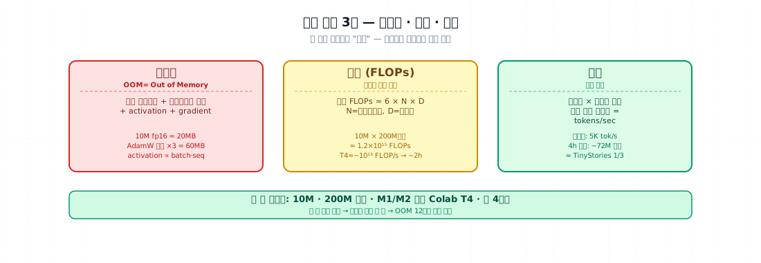
Three axes of trainability — memory, compute, time

1. Concept — three axes you must all pass¶

Training is feasible only if you clear all three at once.

Axis	What determines it	Failure signal
Memory	Model size + optimizer state + activations	OOM (out of memory)
Compute (FLOPs)	Token count × model size	Training that never finishes
Time	A function of the two above	Blows past your deadline

The classic trap: memory passes, time doesn't. You can load a 10B quantized model on a laptop for inference — but training it is another matter. Check all three before you start.

2. Why it matters — "just try it" doesn't work here¶

Once training starts, stopping early means losing everything since the last checkpoint. Run 12 hours on a laptop, hit an OOM, and you lose 12 hours. A five-minute estimate up front pays for itself.

There's also an intentional ratio between model size and training data. A model starved of data (under-trained) underperforms. A tiny model fed far more data than it can benefit from either overfits or saturates. The balance matters.

3. Where it's used — the Chinchilla law and SLM's deliberate departure¶

Chinchilla (Hoffmann et al., 2022) in one line¶

Given a fixed compute budget, scale model size N and training tokens D together. The empirical optimum is roughly:

\[ D \approx 20 \times N \]

(1B parameters → ~20B tokens is compute-optimal.)

Why SLMs ignore this¶

Apply Chinchilla to the 10M model in this book: 200M tokens. That actually matches 20×. But for most deployed SLMs, inference cost matters more than training cost — so it's worth spending more on training to squeeze more capability out of each inference token. That's why SLMs deliberately over-train:

Model	Parameters	Training tokens	Ratio	Approach
Chinchilla 70B	70B	1.4T	20×	Compute-optimal
Llama 3 8B	8B	15T	~1900×	Heavy over-training
SmolLM2 1.7B	1.7B	11T	~6500×	Heavier over-training
This book 10M	10M	200M	20×	Balanced (time-constrained)

This book stops at 20× only because of time. If you have more hours, push to 100× — the model keeps improving.

4. Minimal example — memory math in 30 seconds¶

Memory during training (rough formula):

\[ \text{Memory} \approx N \times (\text{params} + \text{grads} + \text{Adam}_1 + \text{Adam}_2 + \text{activations}) \]

Each term in bytes:

Term	bf16/fp16	fp32
params	2N	4N
grads	2N	4N
Adam m (1st moment)	4N	4N
Adam v (2nd moment)	4N	4N
Adam total	12N + 2 (params)	16N
activations	batch × seq × hidden (function of shape)	same

With bf16 + Adam + grads, expect roughly 14–16 bytes/param plus activations. Examples:

10M model → params/grads/optimizer ≈ 160 MB + 100–500 MB activations → ~1 GB total. M2 (16 GB) and T4 (16 GB) both comfortable.
125M model (GPT-2 small) → ~2 GB + 1–3 GB activations → 3–5 GB. T4 fine, mobile not.
1B model → ~16 GB + activations → 20 GB+. T4 (16 GB) can't train it; needs A100.

memory_budget.py
def training_memory_gb(N_params, dtype="bf16"):
    """Rough training memory estimate (excludes activations)."""
    bytes_per_param = 2 if dtype in ("bf16", "fp16") else 4
    # bf16 mixed: params + grads = 2+2, Adam = 4+4 = 12, total ~14
    # fp32 pure : 4+4+4+4 = 16
    factor = 14 if dtype in ("bf16", "fp16") else 16
    return N_params * factor / 1e9  # GB

for N, name in [(1e7, "10M"), (1.25e8, "125M"), (1e9, "1B"), (7e9, "7B")]:
    print(f"  {name:5s}  bf16: {training_memory_gb(N, 'bf16'):6.2f} GB")

5. Hands-on tutorial — baseline math for this book¶

Time = total FLOPs / device throughput¶

FLOPs per token for one training step (forward + backward):

\[ \text{FLOPs/token} \approx 6N \]

(forward ≈ 2N, backward ≈ 4N — standard approximation from Kaplan et al., 2020)

Total FLOPs for a training run:

\[ \text{Total} \approx 6 \times N \times D \]

For this book (10M params, 200M tokens):

\[ 6 \times 10^7 \times 2 \times 10^8 = 1.2 \times 10^{16} \text{ FLOPs} \]

Effective throughput per device (real mixed-precision training, including memory bandwidth and data loading — typically 30–50% of the spec):

Device	Spec (TFLOPS bf16)	Effective (TFLOPS)	This book's training time
M2 (CPU)	~0.5	0.2	~17 hours
M2 Pro (MPS, GPU cores)	~7	3	~1.1 hours
Colab T4	65	20	~10 minutes
Colab A100	312	150	~1.5 minutes

The gap between spec and effective throughput comes from data loading, memory bandwidth, and non-tensor operations. 30–50% is a conservative estimate.

Baseline: M2 Pro MPS or Colab T4 finishes the book's baseline run in tens of minutes to one hour. The "4 hours" in the title is a conservative estimate that includes toolchain setup, evaluation, and debugging.

Compute it yourself¶

time_budget.py
def hours_to_train(N_params, D_tokens, effective_tflops):
    flops = 6 * N_params * D_tokens
    seconds = flops / (effective_tflops * 1e12)
    return seconds / 3600

scenarios = [
    ("10M  · 200M  · M2 Pro MPS", 1e7,   2e8,  3),
    ("10M  · 200M  · T4",         1e7,   2e8,  20),
    ("30M  · 600M  · T4",         3e7,   6e8,  20),
    ("125M · 2.5B  · T4",         1.25e8, 2.5e9, 20),
    ("125M · 2.5B  · A100",       1.25e8, 2.5e9, 150),
]
for name, N, D, tf in scenarios:
    print(f"  {name:35s}  {hours_to_train(N, D, tf):6.2f} h")

Expected output:

10M  · 200M  · M2 Pro MPS              1.11 h
10M  · 200M  · T4                      0.17 h
30M  · 600M  · T4                      1.50 h
125M · 2.5B  · T4                     10.42 h
125M · 2.5B  · A100                    1.39 h

Takeaways:

The book's baseline (10M · 200M) finishes comfortably on anything.
Pushing to 30M · 600M (same Chinchilla ratio) still fits on a free Colab T4 in 1.5 hours — well under the 12-hour session limit.
125M (GPT-2 small) starts straining the T4. You'd want an A100 or multiple T4s.

6. Common pitfalls¶

1. Forgetting activation memory. "params + grads + Adam = 14N" is only the weight memory. Increase batch size without checking activations and you'll OOM. Activations scale as batch × seq × hidden × ~12. At seq=512, hidden=256, batch=16, activations alone are ~1.5 GB.

2. Trusting spec FLOPs. A100 spec is 312 TFLOPS for fp16 dense matrix multiplication at peak. Real training is dominated by memory bandwidth, communication, and data loading. Effective ≈ spec × 0.4 is safe.

3. Free Colab session cuts. T4 availability isn't guaranteed. Sessions drop frequently during long runs. Without checkpoints (Ch 14), a 7-hour run lost to a disconnect is just 7 hours gone.

4. PyTorch MPS op fallback on Apple Silicon. Some ops — particularly newer attention variants — fall back to CPU on MPS. When that happens, you go from ~7 TFLOPS to 1/100 of that. Before a long run, verify with torch.backends.mps.is_available() and measure actual tokens/sec on a 100-step warmup.

5. Confusing token count with step count. step = D_tokens / (batch × seq_len × grad_accum). Chinchilla's law is stated in tokens D, not steps.

7. Production checklist¶

30-second pre-training checklist:

Memory — training_memory_gb(N) + activation estimate + 30% margin → fits in device RAM?
Time — hours_to_train(N, D, tflops) → fits in your schedule?
Checkpoints — saving every 30 minutes or 1,000 steps? (Ch 14)
Colab — saved to mounted Drive in case of disconnect? Aware of the 12-hour free-tier limit?
Data — D tokens tokenized, shuffled, and cached?
Eval set — 1–2% held out separately? (Part 5)

If the math doesn't pass:

Memory over budget → smaller model or smaller batch + gradient accumulation (Ch 13)
Time over budget → reduce both model and token count or rent an A100 (Colab Pro)
Both tight → improve data quality to need fewer tokens (Part 2 Ch 7)

8. Exercises¶

Write down your laptop's RAM, CPU, and GPU specs. Use training_memory_gb to estimate the largest model you can train. Include a 30% activation margin.
How long would 30M model + 600M tokens (Chinchilla ratio) take on your hardware? Use hours_to_train. Does it fit in 12 hours?
The 30–50% effective-vs-spec gap is a rule of thumb. Run a small training job (10M model, 1,000 steps) on your device and measure actual tokens/sec. What percentage of spec does it reach?
(Think about it) What happens to memory and time if you intentionally over-train at 100× — 10M model, 1B tokens? Which axis hits its limit first?

Next¶

Now you know your hardware ceiling. The next chapter surveys the existing open-weight SLMs — their sizes, dense vs MoE structure, and where the 10M model you'll build sits among them.

Next → Ch 4 The Open-Weight SLM Landscape

Sources¶

Hoffmann et al. (2022). Training Compute-Optimal Large Language Models. (Chinchilla) arXiv:2203.15556
Kaplan et al. (2020). Scaling Laws for Neural Language Models. arXiv:2001.08361 — source of the 6N approximation
HuggingFace SmolLM2 blog — over-training ratios
Llama 3 model card — 8B / 15T tokens
PyTorch MPS backend docs (Apple Silicon)