nanoGPT in 100 Lines

What you'll learn
- The Ch 8 attention + Ch 9 modern blocks assembled into a GPT-mini in one file (~100 lines)
- The block → layer → model composition pattern — the base for all Part 4 training code
- Following Karpathy's nanoGPT spirit: "minimum dependencies, entire model in one screen"
Prerequisites
Ch 8 Attention — SDPA. Ch 9 — RoPE and RMSNorm concepts. You should have built at least one nn.Module before.
Credit
The code in this chapter is based on the spirit of Karpathy's nanoGPT and minGPT. Variable names and structure are rewritten for this book's style, but the ideas are his.
1. Concept — The Whole Model in One File
Large libraries (transformers, fairseq) are deeply abstracted. When you're learning, the flow gets hidden. nanoGPT is the opposite — single file, only PyTorch, whole model in one screen. That's optimal for learning.
This book's GPT-mini follows the same spirit:
| Component | Lines | Role |
|---|---|---|
RMSNorm |
8 | Straight from Ch 9 |
apply_rope |
6 | Straight from Ch 9 |
CausalSelfAttention |
22 | Ch 8 + RoPE |
FFN (SwiGLU option) |
10 | Straight from Ch 9 |
Block (Norm → Attn → Norm → FFN) |
14 | Two residuals |
GPTMini (embedding + N×Block + lm_head) |
25 | Full model |
| Total | ~85 |
The training loop is in Part 4. This chapter is about the model class itself.
2. Why This Structure — Two Residuals per Block
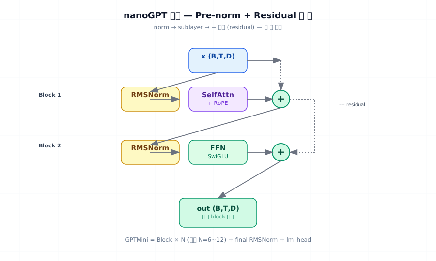
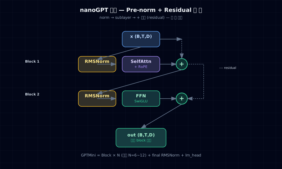
The standard transformer decoder block:
Pre-norm + residual, twice. Two key facts:
- Residual connections allow gradients to flow even through many layers.
- Pre-norm (normalizing before the sublayer) keeps training stable. Post-norm breaks around 100 layers.
Stack this block N times and you have a model.
3. Where This Is Used
- The base for Part 4 training — the next four chapters train this exact class.
- The evaluation target in Part 5 — perplexity and sample review.
- The quantization and GGUF target in Part 6 — converting trained weights.
- The capstone starting point — domain SLM begins here.
4. The Full Code — ~100 Lines
| nano_gpt.py | |
|---|---|
1 2 3 4 5 6 7 8 9 10 11 12 13 14 15 16 17 18 19 20 21 22 23 24 25 26 27 28 29 30 31 32 33 34 35 36 37 38 39 40 41 42 43 44 45 46 47 48 49 50 51 52 53 54 55 56 57 58 59 60 61 62 63 64 65 66 67 68 69 70 71 72 73 74 75 76 77 78 79 80 81 82 83 84 85 86 87 88 89 90 91 92 93 94 95 96 97 98 99 100 101 102 103 104 105 106 107 108 109 110 111 112 113 114 115 116 117 118 119 120 121 122 123 124 125 126 127 128 129 130 131 132 133 134 135 136 137 138 | |
- RoPE applies just before attention, after splitting into heads. Same formula as Ch 9.
- Split into heads → apply RoPE → SDPA. FlashAttention is included automatically.
- Pre-norm: norm → sublayer → residual, twice. The Ch 9 recommendation.
- Weight tying — input and output embeddings share the same weight matrix. Saves parameters and stabilizes training (Press & Wolf, 2017).
- Context window guard — use only the most recent
max_lentokens.
5. In Practice — Run It Once
Typical output:
What to verify:
- Parameter count is ~10M — matches this book's target.
- Pre-training loss is ~ln(vocab) = ln(8000) ≈ 8.99 — sanity check passes. A uniform distribution over 8000 tokens has this cross-entropy.
- Generation output is random noise since the weights aren't trained. After Part 4, loss will drop from 8.99 toward ~4.
6. Common Failure Modes
1. Recomputing the RoPE table every forward — Use register_buffer to compute it once. CPU↔GPU movement is also handled automatically.
2. Not using weight tying — This adds vocab_size × d_model extra parameters. With 8K vocab and d_model=256, that's 2M extra — 20% of a 10M model.
3. RMSNorm gamma initialized to 0 — Model won't train. Initialize to 1.0 (torch.ones).
4. Using attention dropout during training — For small models (10M), dropout hurts more than it helps. Add dropout only for larger models, at ~0.1.
5. nn.Linear(bias=True) default — Standard transformers use no bias. Explicitly set bias=False.
6. cos[:T] can't broadcast over batch — apply_rope broadcasts (T, head_dim/2) over (B, H, T, head_dim/2). PyTorch handles this, but if you get a shape mismatch after modification, add .unsqueeze(0).unsqueeze(0).
7. No KV cache during generation — Each new token requires a full forward pass from scratch. Fine for this chapter, but Part 6 adds KV caching for production inference.
7. Operational Checklist
- Print parameter count — sanity check every time you change config
- Pre-training loss ≈ ln(vocab) — confirms correct model initialization
- Small input (B=2, T=8) forward pass — shape verification
-
model.eval()mode disables dropout — verify - RoPE table via
register_buffer— automatically included in model save (persistent=Falseexcludes it) - Config as a dataclass — easy dict conversion for experiment tracking, reproducibility
8. Exercises
- Run the code as-is and record the parameter count and pre-training loss on your own hardware. Does it match ln(8000) ≈ 8.99?
- Set
n_layer=12andd_model=384. How many parameters does it have? Use thetrain_mem_gbformula from Ch 3 to check if it's trainable on your machine. - Replace SwiGLU with a standard GeLU FFN (
hidden = 4 × d_model). How do parameter count and pre-training loss compare? - Remove weight tying (
self.lm_head.weight = self.tok_emb.weightline). How much does the parameter count increase? - (Think about it) nanoGPT deliberately limits dependencies to PyTorch only. Why? Write one paragraph on the tradeoffs between learning-oriented code and production code.
References
- Karpathy. nanoGPT — https://github.com/karpathy/nanoGPT
- Karpathy. minGPT — https://github.com/karpathy/minGPT
- Press & Wolf (2017). Using the Output Embedding to Improve Language Models. arXiv:1608.05859 — weight tying
- Touvron et al. (2023). Llama — standardized pre-norm + RMSNorm + RoPE + SwiGLU