Monitoring · Feedback Loop · Cost

What you'll learn

• Quality signals — refusal rate, re-ask rate, hallucination, self-consistency
• Drift — detecting shifts in input distribution (KL divergence)
• Feedback loop — user corrections flowing into the next training cycle
• Cost model — GPU time / API tokens / labeling / license / 1-year ROI
• Rollback strategy — adapter swap in under 30 seconds

Prerequisites

Ch 30 Regression Eval, Ch 31 Serving. This chapter is the final gate of production operations.

---

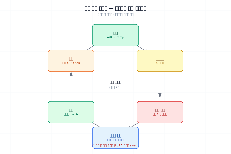
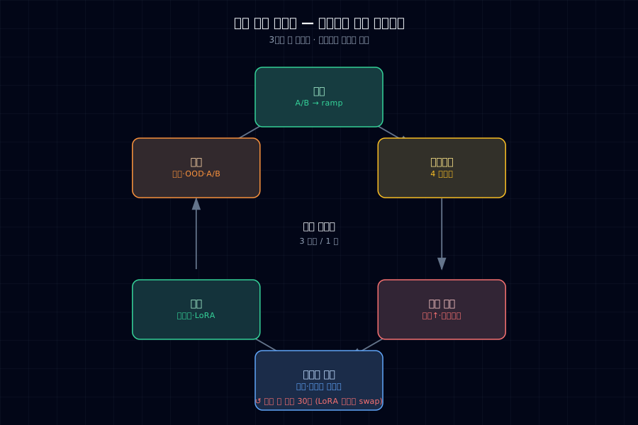
1. Concept — The Production Cycle

Deploy → Monitor → Detect signal → Collect data → Train → Evaluate → Deploy
                                                                ↑ ── quarterly (3 months) ── ↓

One cycle per quarter. Each stage driven by automated signals.

---

2. Quality Signals — 4 Types

(1) Refusal rate

The fraction of responses where the model said "I don't know" or refused to answer. A sudden spike means alignment is broken or OOD input has increased.

def is_refusal(text):
    keywords = ["잘 모르겠", "도와드릴 수 없", "I don't know", "I cannot"]
    return any(k in text for k in keywords)

refusal_rate = sum(is_refusal(r) for r in responses) / len(responses)

(2) Re-ask rate

The same user submits a similar question again within 30 seconds — a signal that the previous answer was unsatisfactory.

(3) Hallucination signal

Self-consistency — ask the same question 5 times. If the answers diverge, something is wrong.

def self_consistency(model, q, k=5):
    answers = [run(model, q, temperature=0.7) for _ in range(k)]
    similarities = [...]    # pairwise BERT score, etc.
    return mean(similarities)    # low score → hallucination risk

(4) User satisfaction (thumbs up/down)

Explicit feedback in the UI. The strongest signal, but response rates are only 1–5%, so it's noisy.

---

3. Drift — Input Distribution Shift

The gap between what the model saw during training and what it sees in production.

from collections import Counter
import math

def drift_kl(train_tokens, prod_tokens, vocab_size):
    """KL divergence — compare token frequencies."""
    train_counts = Counter(train_tokens)
    prod_counts = Counter(prod_tokens)
    train_total = sum(train_counts.values())
    prod_total = sum(prod_counts.values())
    kl = 0
    for tok in set(train_counts) | set(prod_counts):
        p = (prod_counts[tok] + 1) / (prod_total + vocab_size)
        q = (train_counts[tok] + 1) / (train_total + vocab_size)
        if p > 0: kl += p * math.log(p / q)
    return kl

KL	Interpretation
< 0.1	Distributions match
0.1–0.5	Slight shift
> 0.5	Drift — consider retraining

The fairy-tale model in this book drifts slowly (few new words). A domain like a call center drifts fast — new products and policy changes shift the distribution quickly.

---

4. Feedback Loop — Production → Training

User corrections and refusals feed into the next training cycle.

Production logs → extract refusals, re-asks, thumbs-down cases
        ↓
PII masking (Ch 29) + IAA validation
        ↓
Added to next cycle's training data + regression suite

Quarterly cycle (3 months):

Timing	Work
Week 1	New model canary (Ch 30)
Week 2	A/B ramp to 100%
Month 1	Monitoring + feedback collection
Month 2	Label refusal/re-ask cases + IAA
Month 3	New training data + train + evaluate
(Next cycle week 1)	New model canary

---

5. Cost Model — 1-Year ROI

Hypothetical operating cost for this book's capstone model (Qwen 0.5B + LoRA):

Item	Cost (monthly)
GPU serving (T4 via vLLM)	$200
Quarterly retraining (Colab Pro)	$50 / quarter
Labeling + synthesis (Haiku)	$50
License	$0 (Apache)
Monitoring infra (Grafana, etc.)	$50
Total	~$300/month = $3,600/year

Compare that to calling the Claude Sonnet API for the same workload:

100,000 calls/month × avg 1,500 tokens × $3/M = $450/month → $5,400/year

→ Self-hosted saves $1,800/year. The one-time training cost (time through the capstone) is separate.

A positive ROI depends on high traffic, PII requirements (you can't send data to an external API), or latency needs (sub-100ms rules out API round-trips).

---

6. Rollback Strategy — Under 30 Seconds

When a production problem is detected:

Action	Time	Impact
Adapter swap (LoRA)	30 s	Zero downtime
Container restart	1 min	Brief 5xx
Base model replacement	10 min	Short downtime

The value of keeping LoRA adapters separate — the decision you made in Ch 24 and Ch 26 pays off here.

# Roll back from adapter v2 to v1
client.set_lora("adapter_v1")        # vLLM API
# Or reroute all traffic to a different adapter

---

7. Common Failure Modes

1. Deploying without monitoring — users close the tab and there's no signal. You need active measurement.
2. Not measuring drift — perplexity suddenly explodes 6 months in. Measure drift weekly.
3. No automated feedback loop — a person reviewing logs every week will eventually stop. Automate extraction + re-run IAA.
4. Not tracking costs — assuming self-hosted is cheaper than an API. In reality: GPU cost + training cost + labeling cost.
5. No rollback strategy — a bad new model means 30 minutes of downtime for a base model redeployment. Adapter swap: 30 seconds.
6. Quarterly cycle stretched to 6 months — you can't keep up with market changes. 3 months is the standard.
7. Judging hallucination by self-consistency alone — the model can be consistently wrong. You still need factual verification.

---

8. Operational Checklist — Year-End Graduation Gate

After completing this book, your model has all of the following:

• Dashboard for 4 signals: refusal rate, re-ask rate, hallucination, thumbs up/down
• KL drift measured weekly
• Automated feedback loop (logs → next training data)
• 1-year cost model + ROI calculation
• 30-second rollback (adapter swap)
• One complete quarterly production cycle
• New model canary + A/B (Ch 30) + ramp
• Regression / OOD / adversarial CI automation

---

9. Exercises

1. Simulate one week of production logs for your model. Build a dashboard of the 4 signals.
2. Measure KL divergence between your training data and simulated production input.
3. Automate the feedback loop — take 100 refusal cases and add them to the next training dataset.
4. Write a 1-year cost model for your domain (self-hosted vs. API).
5. (Think about it) Is "retrain every quarter" always right? What reasons might you have to skip a retraining cycle?

---

Part 8 Wrap-up

Chapter	What it covers
Ch 29	Data pipeline (PII, synthetic labels, IAA)
Ch 30	Regression, OOD, adversarial, A/B
Ch 31	Serving (llama.cpp / vLLM / latency budget)
Ch 32	Monitoring, feedback loop, cost, rollback

---

Book Graduation — 32 Chapters Complete

Reaching this point means:

• Built a 10M SLM from scratch (Parts 1–6)
• Picked an existing sLLM and applied LoRA (Part 7)
• Capable of production operations: PII, evaluation, serving, monitoring (Part 8)
• Published your model to HuggingFace Hub (Capstone)

The original question — "why do open-weight models come in different sizes?" — you now have the answer. You built the reasons yourself.

Next → Capstone. Run the full cycle one more time and put your own model out into the world.

---

References

• "Designing Machine Learning Systems" (Chip Huyen) — monitoring and feedback loop chapter
• Anthropic / OpenAI production eval patterns (blog posts)
• Google SRE — progressive rollout and rollback
• HuggingFace evaluate · Langfuse · Weights & Biases