Attention Revisited

What you'll learn

• Scaled dot-product attention — the equation in one line, the code in five
• Why causal masking is necessary (the core constraint in generative models)
• PyTorch's F.scaled_dot_product_attention one-liner — verifying it matches the manual version
• Multi-head is just a reshape — it's not a new algorithm

Prerequisites

A feel for matrix multiplication, the definition of softmax, basic PyTorch tensor operations. If you've seen attention before, even better — this chapter is about coding it again by hand, not first contact.

---

1. Concept — The Equation

\[ \text{Attention}(Q, K, V) = \text{softmax}\!\left(\frac{Q K^\top}{\sqrt{d_k}}\right) V \]

All three inputs have the same shape — (seq, d_k). The output is also (seq, d_k).

Intuition: each token scores every other token, then uses those scores to take a weighted average of values. It's a differentiable answer to "which positions should I pay attention to when generating this token?"

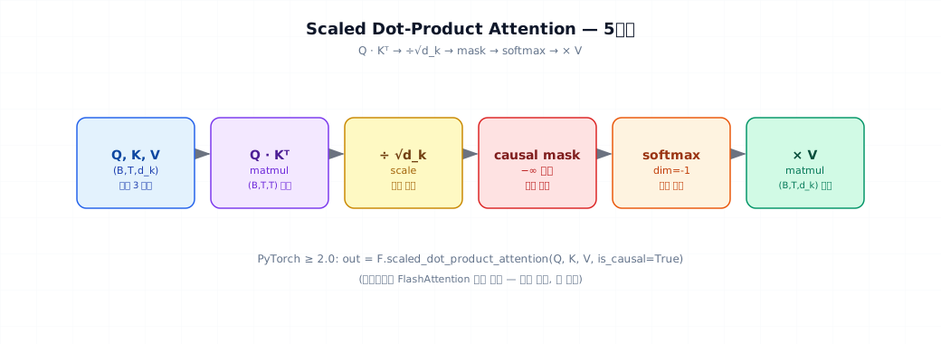
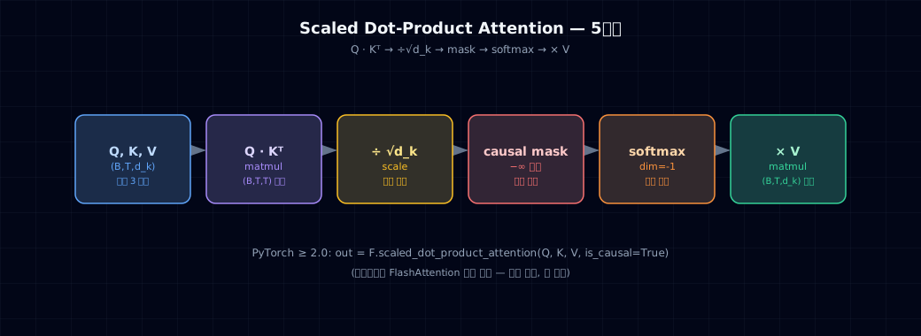
Five steps:

1. Q · Kᵀ — how much does token i care about token j? Produces a (seq, seq) score matrix.
2. ÷ √d_k — stabilize the score variance. Without this, large d_k values push dot products too large, causing softmax to spike to one position.
3. Causal mask — set future positions to -∞ (generative models only).
4. Softmax — convert to a probability distribution.
5. × V — weighted sum of values.

---

2. Why It Replaced RNNs and CNNs

Approach	"What can it see?"	Distance dependency	Parallelizable
RNN	Previous hidden state only (distant tokens reached indirectly)	O(n) hops	No (sequential)
CNN	Within a fixed window (e.g., 3–7)	Window-limited	Yes
Attention	Every position directly	O(1)	Yes (matmul)

Direct access to any position + full parallelization. Those two properties are why transformers replaced RNNs and CNNs.

The cost: O(n²) memory — Q · Kᵀ is (seq, seq). At seq=4K, that matrix alone is 64MB (fp32). FlashAttention (§5) addresses this.

---

3. Where It's Used

• Every transformer layer — encoder, decoder, and cross-attention all use the same equation.
• GPT-style (decoder-only) — causal mask applied. This is the model we're building.
• BERT-style (encoder-only) — no mask (bidirectional).
• T5 (encoder-decoder) — encoder: no mask; decoder: causal + cross-attention.

This book covers causal self-attention only (Part 7 Ch 25 touches encoders, Ch 28 covers encoder-decoders briefly).

---

4. Minimal Example — 30 Lines by Hand

import torch
import torch.nn.functional as F

torch.manual_seed(0)
B, T, D = 1, 4, 8                          # batch, seq, hidden
x = torch.randn(B, T, D)

# Learnable projections — real models use nn.Linear; here exposed for clarity
Wq = torch.randn(D, D); Wk = torch.randn(D, D); Wv = torch.randn(D, D)
Q = x @ Wq                                 # (B, T, D)
K = x @ Wk
V = x @ Wv

scores = Q @ K.transpose(-2, -1)           # (B, T, T)        (1)
scores = scores / (D ** 0.5)               #                  (2)

# Causal mask: position i can't see j > i
mask = torch.triu(torch.ones(T, T), diagonal=1).bool()  # (T, T)  (3)
scores = scores.masked_fill(mask, float('-inf'))

attn = F.softmax(scores, dim=-1)           # (B, T, T)
out = attn @ V                             # (B, T, D)         (4)
print("attention weights row 0:", attn[0, 0])  # position 0 only sees itself -> [1, 0, 0, 0]

1. Q @ K.T — dot product for every pair (i, j). Shape (seq, seq).
2. Divide by √d_k — the key trick. Without it, softmax becomes either flat or spiky as d grows.
3. triu(diagonal=1) — True above the main diagonal. Filling those positions with -∞ makes softmax output 0 there. Only positions j ≤ i are visible.
4. Weighted sum of values using attention weights. Output is the same shape as input.

Typical output:

attention weights row 0: tensor([1., 0., 0., 0.])  # position 0
attention weights row 1: tensor([0.31, 0.69, 0., 0.])  # position 1
attention weights row 2: tensor([0.20, 0.45, 0.35, 0.])  # position 2

Position i always attends only to 0..i — the definition of causal.

---

5. In Practice — Comparing with F.scaled_dot_product_attention

Since PyTorch 2.x, F.scaled_dot_product_attention does the same operation in one call. Internally, it auto-selects FlashAttention (Dao et al., 2022) or another efficient implementation.

import torch
import torch.nn.functional as F

torch.manual_seed(0)
B, T, D = 1, 4, 8
x = torch.randn(B, T, D)
Wq = torch.randn(D, D); Wk = torch.randn(D, D); Wv = torch.randn(D, D)
Q, K, V = x @ Wq, x @ Wk, x @ Wv

# One line                                                       (1)
out_fast = F.scaled_dot_product_attention(Q, K, V, is_causal=True)

# Manual version                                                 (2)
mask = torch.triu(torch.ones(T, T), diagonal=1).bool()
scores = (Q @ K.transpose(-2, -1)) / (D ** 0.5)
scores = scores.masked_fill(mask, float('-inf'))
out_manual = F.softmax(scores, dim=-1) @ V

print("max abs diff:", (out_fast - out_manual).abs().max().item())  # ~1e-6

1. is_causal=True applies the mask automatically. Shape inference is automatic too — the 5 lines you wrote collapse to one.
2. Results should match. Differences below 1e-6 are floating-point rounding.

Why use the one-liner:

• Speed: On GPU, FlashAttention uses O(n) memory instead of O(n²). You'll feel the difference from seq=2K onward.
• Memory: The full attention matrix never materializes in memory.
• Maintenance: Future PyTorch upgrades automatically make it faster.

When to write it by hand: debugging, attention weight visualization (Ch 18), implementing a new variant (parts of RoPE).

---

6. Multi-Head — It's Just a Reshape

With d_model=64, n_head=8, each head has head_dim=8. Each head attends independently, then results are concatenated.

B, T, D, H = 1, 4, 64, 8
head_dim = D // H                           # 8

# (B, T, D) -> (B, T, H, head_dim) -> (B, H, T, head_dim)
def split(x):
    return x.view(B, T, H, head_dim).transpose(1, 2)

Q, K, V = split(Q), split(K), split(V)                          # (1)
out = F.scaled_dot_product_attention(Q, K, V, is_causal=True)    # auto broadcasts (2)
out = out.transpose(1, 2).contiguous().view(B, T, D)             # merge back

1. view + transpose — two lines. Not a new algorithm — just splitting a dimension.
2. SDPA auto-broadcasts over the head dimension. Each head attends independently.

Why split into heads: the model can learn multiple "views" simultaneously. Head 1 might focus on the immediately previous token; head 2 might track the last noun. You can verify this with visualization after training (Ch 18).

---

7. Common Failure Modes

1. Forgetting √d_k — Loss doesn't decrease in early training. At d_k=64, dot products are on average √64=8× larger than expected, causing softmax to spike.

2. Wrong mask shape — The causal mask is (T, T). If attention scores are (B, H, T, T), broadcasting handles the standard case automatically — but if you add padding masks or other variants, you'll need to match shapes manually.

3. Filling the mask with 0 instead of -inf — Before softmax, the fill value must be -inf. Softmax converts -inf to 0 probability. Filling with 0 gives the wrong result.

4. dtype mismatch — Q, K, V in fp16 but mask in fp32 causes a cast. Add .to(Q.dtype).

5. Using is_causal=True and a manual mask at the same time — SDPA may apply the mask twice. Use one or the other.

6. Using .T on multi-dimensional tensors — .T reverses all dimensions. Always use transpose(-2, -1) for safety.

---

8. Operational Checklist

• Use F.scaled_dot_product_attention (manual implementation for debugging only)
• PyTorch ≥ 2.0 — FlashAttention selected automatically
• For long sequences: is_causal=True avoids materializing the mask in memory
• head_dim should be a multiple of 16 (Tensor Core efficiency) — typically 32, 64, or 128
• KV cache for inference — separate concern (Ch 11 memory math + Part 6)
• Attention weight visualization: use a hook after training — don't store weights inside forward (memory explosion)

---

9. Exercises

1. Run the §4 five-line attention with batch B=2, seq T=8, hidden D=16. Verify the attn shape and that each row sums to 1 (attn.sum(-1)).
2. Compare the SDPA one-liner vs. the manual version across dtypes (fp32, fp16, bf16). Which dtype shows the largest difference?
3. Flip the causal mask (triu(diagonal=0) — can only see current and future, not past) and compare the loss curve after one epoch against the correct mask.
4. Initialize all 8 heads with identical weights. What happens? Why does PyTorch's default initialization guarantee different results per head?
5. (Think about it) At seq=10K, attention's O(n²) memory hits 100MB. At seq=100K, that's roughly 10GB. How does FlashAttention solve this? Explain in one paragraph.

---

References

• Vaswani et al. (2017). Attention Is All You Need. arXiv:1706.03762
• Dao et al. (2022). FlashAttention: Fast and Memory-Efficient Exact Attention with IO-Awareness. arXiv:2205.14135
• PyTorch docs — torch.nn.functional.scaled_dot_product_attention
• Karpathy. Let's build GPT (YouTube, 2023) — the same 5 lines on video