Parameter and Memory Math

What you'll learn
- Compute parameter count by hand from a config — breaking down embedding, attention, and FFN
- Training memory = params + gradients + optimizer state + activations — the formula and the arithmetic
- Inference memory = params + KV cache — as a function of seq, layers, and heads
- Exact estimates for this book's 10M / 30M / 125M models
Prerequisites
Ch 10 nanoGPT code structure. Ch 3 Laptop Budget's memory formula (14N) — this chapter breaks it down.
1. Concept — Where Does Memory Go?
During one training step:
| Component | What it stores | Size |
|---|---|---|
| params | Model weights | 2N (bf16) |
| grads | Gradient per parameter | 2N |
| Adam m | 1st moment (per param) | 4N (fp32 recommended) |
| Adam v | 2nd moment | 4N |
| activations | Intermediate tensors from forward pass, kept for backward | f(B, T, D, L) |
Everything except params is either a function of N or a function of batch and sequence length. Increase any axis and memory goes up proportionally.
Inference is lighter — only params + KV cache.
2. Why You Need the Math
If training runs out of memory, you lose 100% of whatever compute time you spent. Thirty seconds of arithmetic before hitting start can prevent that.
Also: same N=10M with different configs means different memory. For example:
- (n_layer=6, d_model=256, max_len=512) → light activations
- (n_layer=2, d_model=512, max_len=2048) → same N, but 4× heavier activations
Do the breakdown before fixing your config.
3. Where This Matters in the Book
- This chapter — estimate for this book's 10M model
- Part 4 Ch 13 — mixed precision and gradient accumulation cut memory by 1/2–1/4
- Part 6 — int4 quantization cuts inference memory by 1/4
- Part 7 Ch 23 — deciding which LoRA base model fits on a laptop
4. Parameter Count Breakdown
Breaking down GPTMini's parameters:
Embedding
nn.Embedding(vocab, D) — vocab × D.
- This book: 8000 × 256 = 2.05 M.
With weight tying (Ch 10), lm_head shares the same weights — no double counting.
Attention (per layer)
qkv: Linear(D, 3D) + proj: Linear(D, D). No bias.
- Per-layer attention = 4 × D².
FFN (per layer, SwiGLU)
w1, w3: Linear(D, H) + w2: Linear(H, D). H = (8/3) × D ≈ 2.67D.
- Per-layer FFN = 3 × D × H ≈ 8 × D².
Norm (per layer)
RMSNorm has one gamma: (D,) parameter. Applied before attention and before FFN — twice — so 2D total per layer. Negligible.
Per-Layer Total
attention 4D² + FFN 8D² + norm 2D ≈ 12 × D².
Full Model
(lm_head not included due to weight tying)
This Book's Numbers (V=8000, L=6, D=256)
embed:   8000 · 256       = 2,048,000
layers:  6 · 12 · 256²    = 4,718,592
norm:    256              = 256
─────────────────────────────────────
total                     ≈ 6.77 M  (≈ 7M)
Change config to (L=6, D=320):
embed:   8000 · 320       = 2,560,000
layers:  6 · 12 · 320²    = 7,372,800
─────────────────────────────────────
total                     ≈ 9.93 M  (≈ 10M, this book's baseline)
5. Training Memory — Per-Component Arithmetic
bf16 Mixed Precision (Standard)
| Component | bytes/param | 7M model (MB) | 10M (MB) | 125M (MB) |
|---|---|---|---|---|
| params (bf16) | 2 | 14 | 20 | 250 |
| grads (bf16) | 2 | 14 | 20 | 250 |
| Adam m (fp32) | 4 | 28 | 40 | 500 |
| Adam v (fp32) | 4 | 28 | 40 | 500 |
| Total (param portion) | 12+2=14 | 84 | 120 | 1500 |
Activation Memory
Intermediate tensors from the forward pass must be kept for the backward pass. Approximately:
where c is 12–20 (number of intermediate tensors per block, implementation-dependent).
This book's example (B=32, T=512, D=320, L=6, c=14, fp16):
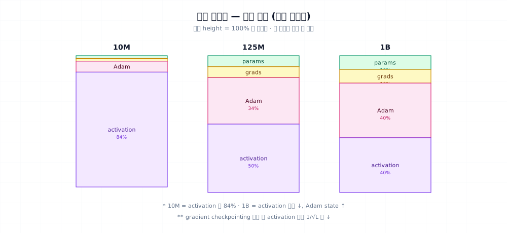
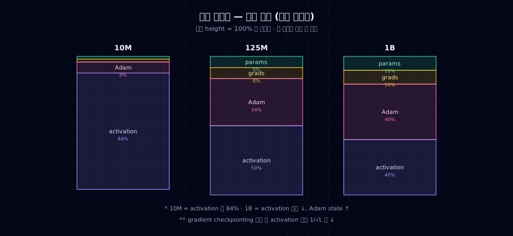
Activations dominate. They can match or exceed the params+optimizer cost.
Gradient Checkpointing
Instead of storing all activations, recompute them during the backward pass. Memory drops to roughly 1/√L (e.g., 840MB → 350MB), at a cost of ~1.3× more compute time. Covered in Part 4 Ch 13.
This Book's 10M Training Memory (Total)
| Component | bf16 | With gradient checkpointing |
|---|---|---|
| params/grads/Adam | 120 MB | 120 MB |
| activations (B=32, T=512) | 840 MB | 350 MB |
| Total | ~1 GB | ~0.5 GB |
M2 (16GB), T4 (16GB), free Colab (12GB) — all comfortable.
Typical output:
6. Inference Memory — KV Cache
At inference time:
(2 = K + V, L=layers, H=heads, d_h=head_dim, T=current seq length, bytes=2 for fp16)
This book's 10M (L=6, H=8, d_h=40, T=1024, fp16):
Negligible. GQA starts to matter at 1B+.
Comparison (Llama-3-8B, T=4K, fp16, GQA):
For large models, the KV cache can rival the model weights.
7. Common Failure Modes
1. Forgetting the embedding — With D=512 and vocab=32K, the embedding alone is 16M parameters. For small models, this can be 30% of total. Don't skip it.
2. Not using weight tying — Embedding counted twice, parameter count doubles for that component. Training also becomes less stable.
3. Setting c=1 in activation estimate — The actual value is 12–20. This causes a 10× estimation error.
4. Adam state in fp16 — Training diverges. Adam state must stay in fp32 (standard for mixed precision training).
5. Forgetting batch size in KV cache — Inference batch=8 means KV cache is 8×. Ties directly to the number of concurrent users.
6. KV cache explosion on length extrapolation — Even if RoPE extrapolation works well, KV cache memory grows 2× or 4× with context length. Memory doesn't extrapolate.
8. Operational Checklist
Before starting training:
-
param_count()— get the exact N -
train_mem_gb(N, B, T, D, L)— estimate training memory - Stay within 70% of device RAM (30% margin)
- Check activation fraction — if >50%, consider gradient checkpointing
- Reduce B or T and recalculate if needed
- Grad accumulation lets you target larger effective batch sizes (Part 4 Ch 13)
For inference:
- KV cache size (function of model + batch + seq length)
- With quantization: params at 1/4, KV cache typically at 1/2 (fp16 → int8)
- Document the context length limit explicitly
9. Exercises
- Compute the parameter count for this book's baseline (V=8000, L=6, D=320) by hand, then verify against
param_count(). - Build two 10M configs: (L=2, D=560) and (L=12, D=180). Compare their training memory. Which is heavier?
- Count the constant
cin your own nanoGPT code by enumerating the intermediate tensors stored during the forward pass. - Compute the KV cache for Llama 3 8B GQA-8 at batch=4, T=8K. How many concurrent users fit on a single A100 80GB?
- (Think about it) Given the same parameter count N, which is more memory-efficient: deep and thin, or shallow and wide? Argue from the activation memory formula.
Part 3 Wrap-Up
| Chapter | What it covers |
|---|---|
| Ch 8 | Attention — one equation, five lines of code |
| Ch 9 | RoPE, RMSNorm, SwiGLU, GQA |
| Ch 10 | nanoGPT — the whole model in one file |
| Ch 11 | Parameter and memory arithmetic |
Next up: Part 4 Training on a Laptop. Time to run the model you built.
References
- Kaplan et al. (2020). Scaling Laws for Neural Language Models. —
6NFLOPs, memory breakdown standard - Rajbhandari et al. (2020). ZeRO: Memory Optimizations Toward Training Trillion Parameter Models. — Adam state decomposition
- Chen et al. (2016). Training Deep Nets with Sublinear Memory Cost. — gradient checkpointing
- nanoGPT's
train.py— memory estimation patterns