Modern Blocks: RoPE, RMSNorm, SwiGLU, GQA¶

What you'll learn

The "why" behind the four blocks that replaced the 2017 original transformer by 2024
RoPE — rotation instead of additive position encoding. Enables length extrapolation.
RMSNorm — drop one term from LayerNorm. Faster, same quality.
SwiGLU — gated activation instead of GeLU. Better expressivity.
GQA — reduce KV heads only. Cuts KV cache memory.
All four differ by 5–10 lines of code. Know them and you can slot them directly into our model.

Prerequisites

Ch 8 Attention — you should be able to picture Q, K, V. Familiarity with LayerNorm and GeLU at a conceptual level.

1. Concept — Why All Four Changed¶

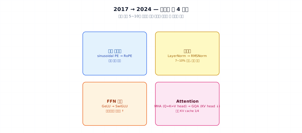
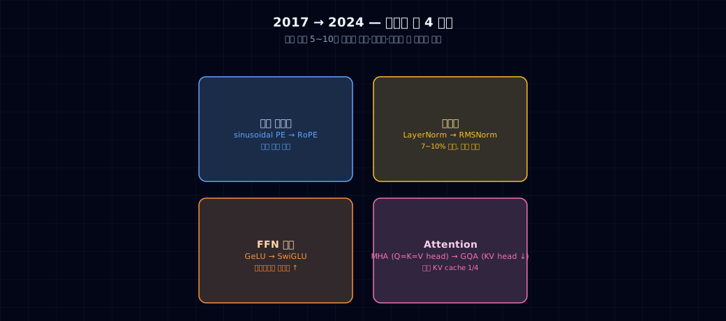
The standard transformer (2017) → the modern standard (2024):

Position	2017	2024 standard
Position encoding	Sinusoidal absolute PE	RoPE
Normalization	LayerNorm	RMSNorm
FFN activation	ReLU → GeLU	SwiGLU
Attention heads	MHA (Q = K = V head count)	GQA

Each change wins on exactly one axis: pure efficiency, inference memory, or length generalization. Training cost is essentially the same.

Four modern blocks — what improved

2. RoPE — Rotary Position Encoding (Su et al., 2021)¶

The Problem with Original PE¶

The original transformer adds sinusoidal PE to the input embeddings. Train on sequences up to length 512 and the model encounters PE patterns it's never seen when you try to run it on longer sequences — performance drops sharply.

RoPE's Idea¶

Instead of adding PE, rotate Q and K. The token at position m has its Q rotated by angle mθ; the token at position n has its K rotated by nθ. The dot product then depends only on (m − n)θ — only the relative distance between tokens matters.

Key effects:

Only relative position matters — absolute position is gone. Extrapolation becomes possible.
No sum with embedding — the embedding + PE sum disappears, making training cleaner.

The Code (5-Line Difference)¶

rope.py
import torch

def precompute_rope(dim, max_len, base=10000.0):
    """Precompute cos/sin table."""
    inv_freq = 1.0 / (base ** (torch.arange(0, dim, 2).float() / dim))   # (dim/2,)
    t = torch.arange(max_len).float()
    freqs = t[:, None] * inv_freq[None, :]                                # (T, dim/2)
    return freqs.cos(), freqs.sin()                                       # both (T, dim/2)

def apply_rope(x, cos, sin):                                              # (1)
    """x: (B, H, T, head_dim). cos/sin: (T, head_dim/2)."""
    x1, x2 = x[..., 0::2], x[..., 1::2]                                   # even/odd split
    rotated_1 = x1 * cos - x2 * sin
    rotated_2 = x1 * sin + x2 * cos
    return torch.stack([rotated_1, rotated_2], dim=-1).flatten(-2)        # (2)

# Usage
cos, sin = precompute_rope(head_dim, max_len)
Q = apply_rope(Q, cos[:T], sin[:T])                                       # same for K
K = apply_rope(K, cos[:T], sin[:T])
# V is not rotated (per the original RoPE definition)

Apply just before attention, after splitting into heads. Q and K only — V stays as-is.
Treat even/odd dimensions as 2D rotation pairs.

Why it became the standard: Llama, Mistral, Qwen, SmolLM2, Phi — nearly every modern SLM uses RoPE. Length extrapolation (e.g., trained on 2K, runs on 8K) is far more stable than sinusoidal PE.

3. RMSNorm — One Term Removed (Zhang & Sennrich, 2019)¶

LayerNorm¶

\[ \text{LN}(x) = \gamma \cdot \frac{x - \mu}{\sqrt{\sigma^2 + \epsilon}} + \beta \]

Computes both mean \(\mu\) and variance \(\sigma^2\). Learns both scale \(\gamma\) and shift \(\beta\).

RMSNorm¶

\[ \text{RMSNorm}(x) = \gamma \cdot \frac{x}{\sqrt{\frac{1}{d}\sum x_i^2 + \epsilon}} \]

Remove the mean subtraction and the shift parameter. Normalize by RMS (root mean square) only.

Why It Works¶

The mean subtraction in LayerNorm turned out to be mostly redundant. Its key effect was variance control. Drop the extra term and you get:

7–10% compute savings (adds up in large models)
Same or better performance

The Code¶

rmsnorm.py
import torch
import torch.nn as nn

class RMSNorm(nn.Module):
    def __init__(self, dim, eps=1e-6):
        super().__init__()
        self.gamma = nn.Parameter(torch.ones(dim))
        self.eps = eps

    def forward(self, x):
        rms = x.pow(2).mean(-1, keepdim=True).sqrt()
        return self.gamma * x / (rms + self.eps)

Adoption: Standard since Llama 1 (2023). GPT-2/3 used LayerNorm.

4. SwiGLU — Gated Activation (Shazeer, 2020)¶

Standard FFN¶

\[ \text{FFN}(x) = W_2 \cdot \sigma(W_1 x) \]

\(\sigma\) was ReLU, then GeLU became standard.

SwiGLU FFN¶

\[ \text{SwiGLU}(x) = W_2 \cdot \big(\text{SiLU}(W_1 x) \odot W_3 x\big) \]

Two projections (\(W_1\) and \(W_3\)): one passes through SiLU, one stays linear. Element-wise product acts as a gate. SiLU = \(x \cdot \sigma(x)\) (multiply by sigmoid).

Why It Works¶

The gate lets the linear layer expand its expressivity nonlinearly. You compensate for the extra weight matrix (\(W_3\)) by reducing the hidden dimension to 2/3 — same parameter count, better performance. Training dynamics are also more stable.

The Code¶

swiglu.py
import torch
import torch.nn as nn
import torch.nn.functional as F

class SwiGLU(nn.Module):
    def __init__(self, dim, hidden):
        super().__init__()
        # Standard FFN has W1, W2. SwiGLU has W1, W2, W3.              (1)
        self.w1 = nn.Linear(dim, hidden, bias=False)
        self.w2 = nn.Linear(hidden, dim, bias=False)
        self.w3 = nn.Linear(dim, hidden, bias=False)

    def forward(self, x):
        return self.w2(F.silu(self.w1(x)) * self.w3(x))                  # (2)

Parameter count increases 1.5× — compensate by reducing hidden from 4× to (8/3)× of dim.
SiLU(W1 x) ⊙ W3 x — gated combination of two projections.

Adoption: Llama, Mistral, Qwen, Phi-3, Gemma 2 — nearly all modern SLMs.

5. GQA — Grouped Query Attention (Ainslie et al., 2023)¶

The KV Cache Problem¶

During inference, every generated token requires caching all previous K and V tensors. Memory:

\[ \text{KV cache} = 2 \cdot L \cdot H \cdot d_h \cdot T \cdot \text{bytes} \]

(2 = K + V, L=layers, H=heads, d_h=head_dim, T=sequence length, bytes=2 for fp16)

For a 7B model (L=32, H=32, d_h=128) at seq=4K in fp16: about 4GB — on top of the 14GB model weights.

GQA's Idea¶

Keep Q heads at 32, reduce K/V heads to 8, and share them across groups. 32 query heads share 8 K/V groups (4:1 ratio).

Memory Savings¶

KV cache scales with the number of K/V heads. Going from 32 → 8 cuts memory by 4×. The same 4K sequence now costs ~1GB.

Variant	Q heads	KV heads	KV cache	Quality
MHA (original)	32	32	4 GB	Baseline
MQA (Multi-Query)	32	1	0.125 GB	Slight degradation
GQA-8	32	8	1 GB	Barely any degradation

The Code Change¶

Before attention, repeat K and V along the head dimension.

gqa.py
def repeat_kv(x, n_rep):
    """x: (B, T, H_kv, d_h). Output: (B, T, H_kv * n_rep, d_h)."""
    B, T, H_kv, d_h = x.shape
    if n_rep == 1:
        return x
    return (x[:, :, :, None, :]
              .expand(B, T, H_kv, n_rep, d_h)
              .reshape(B, T, H_kv * n_rep, d_h))

# Just before attention
n_rep = n_q_heads // n_kv_heads          # 32 / 8 = 4
K = repeat_kv(K, n_rep)
V = repeat_kv(V, n_rep)
# SDPA call is identical from here

Adoption: Started with Llama 2 70B, now standard in Llama 3, Mistral, Qwen2.5, Phi-3, Gemma 2, SmolLM2, and more. This book's 10M model is too small for GQA to matter, but the LoRA base in Part 7 (Qwen2.5-0.5B) uses it.

6. Common Failure Modes¶

1. Applying RoPE to V — RoPE applies to Q and K only. Not to V. Also: apply at the head_dim dimension, not batch or head dimensions.

2. Wrong RoPE base (10000) — When extrapolating beyond training length, scaling the base is standard ("YaRN", "longrope"). Within training length, use the default.

3. RMSNorm position — Modern standard is pre-norm (norm → attention → residual). Post-norm becomes unstable at ~100 layers. All Llama-family models use pre-norm.

4. SwiGLU hidden size — For a fair parameter comparison, hidden = (8/3) × dim (Llama standard). Using 4× dim gives you 1.5× more parameters — not a fair comparison.

5. Changing head count after training — You can't change the number of KV heads after training. Fix it before training starts.

6. Applying all four to a small model — On a 10M model, the effects are negligible or counterproductive. This book recommends RoPE + RMSNorm for 10M, SwiGLU is optional, GQA is not worth it.

7. Operational Checklist¶

Recommended settings for this book's 10M model:

RoPE — length extrapolation + training stability. 5 lines of code.
RMSNorm — 7–10% faster. Same quality. Nearly free.
SwiGLU — optional. ReLU/GeLU is fine for small models.
GQA — skip. Head count is too small to matter.
Pre-norm — training stability. Always.

For Part 7's LoRA base (1B-scale), all four are used. That's the modern SLM standard.

8. Exercises¶

Measure forward pass time for RMSNorm vs. LayerNorm on the same input (B=8, T=512, D=512) over 100 iterations. Do you see the 7–10% savings?
Change RoPE's base=10000 to base=100000, train to the same length, then evaluate on extrapolated lengths (4K → 16K). Which is more stable?
Train a small model (10M, 50M tokens) with SwiGLU using hidden = 4 × dim vs hidden = (8/3) × dim. Compare loss curves.
Calculate KV cache memory for GQA-8 (Q=32, KV=8) vs. MHA (Q=32, KV=32) at seq=2K, 12 layers, head_dim=64, fp16. Show your work.
(Think about it) If someone had proposed all four changes at once in 2017, would the field have adopted them? Why were they introduced one at a time? Write a paragraph from the perspective of how fields evolve.

References¶

Su et al. (2021). RoFormer: Enhanced Transformer with Rotary Position Embedding. arXiv:2104.09864
Zhang & Sennrich (2019). Root Mean Square Layer Normalization. arXiv:1910.07467
Shazeer (2020). GLU Variants Improve Transformer. arXiv:2002.05202
Ainslie et al. (2023). GQA: Training Generalized Multi-Query Transformer Models from Multi-Head Checkpoints. arXiv:2305.13245
Touvron et al. (2023). Llama — standardized all four blocks
Karpathy. nanoGPT's model.py — the same four blocks in under 100 lines