The Training Loop and AdamW

What you'll learn

• The 5 steps of one training step: forward → loss → backward → optimizer → zero_grad
• AdamW — Adam with decoupled weight decay. Why it became the standard
• Cosine schedule + warmup — the learning rate changes over time
• Gradient clipping — prevents divergence. One line.
• Default hyperparameter values for this book's 10M model

Prerequisites

The GPTMini class from Ch 10 nanoGPT. Having called loss.backward() in PyTorch at least once.

---

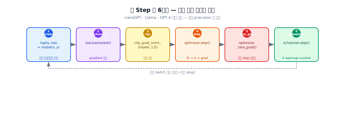
1. The 5 steps of one training step

for batch in loader:
    logits, loss = model(batch.x, batch.y)   # 1. forward
    loss.backward()                          # 2. backward (compute gradients)
    torch.nn.utils.clip_grad_norm_(model.parameters(), 1.0)   # 3. clip
    optimizer.step()                         # 4. update parameters
    optimizer.zero_grad()                    # 5. reset gradients
    scheduler.step()                         # 6. update learning rate

These 6 lines are the core of every training loop. nanoGPT, Llama, GPT-4 — they all follow the same pattern (differing only in distribution and precision).

What each line does:

Step	What	Why
1 forward	input → logits → loss	predict with current parameters
2 backward	derivative of loss w.r.t. each parameter	figure out which direction to move
3 clip	cap gradient norm at 1.0	prevent divergence
4 step	parameter = parameter − lr × grad	take one step
5 zero_grad	set gradients to 0	prevent accumulation into next step
6 scheduler	update lr	warmup → cosine decay

---

2. AdamW — Adam with decoupled weight decay

Adam (Kingma & Ba, 2014)

Adam tracks a first moment (gradient mean) and second moment (gradient squared mean) per parameter. It adapts the step size automatically.

\[ m_t = \beta_1 m_{t-1} + (1-\beta_1) g_t \\ v_t = \beta_2 v_{t-1} + (1-\beta_2) g_t^2 \\ \theta_t = \theta_{t-1} - \frac{\eta \cdot m_t}{\sqrt{v_t} + \epsilon} \]

Adam → AdamW (Loshchilov & Hutter, 2017)

Classic L2 regularization (grad += weight_decay * param) couples with Adam's √v_t denominator, causing larger parameters to be regularized less strongly. AdamW decouples regularization from the gradient update:

\[ \theta_t = \theta_{t-1} - \eta \cdot \left(\frac{m_t}{\sqrt{v_t} + \epsilon} + \lambda \theta_{t-1}\right) \]

Effect: uniform regularization across all parameters. More stable training and better generalization. The standard for every LLM since 2017.

Default values

Item	Value	Notes
lr (peak)	3e-4 ~ 6e-4	higher for smaller models
betas	(0.9, 0.95)	standard for large LLMs (not 0.999)
eps	1e-8	rarely touched
weight_decay	0.1	exclude embeddings and norms

Important: don't apply weight_decay to embeddings or RMSNorm's gamma. Split into two parameter groups in PyTorch.

---

3. Cosine schedule + warmup

The learning rate changes with each step. The standard pattern:

lr
 ↑
 |    ___________
 |   /           \________________
 |  /                             \____
 |_/_______________________________________\__→ step
   |--warmup--|---------cosine decay-----|
       1%~5%            the rest

Warmup (1~5%)

Linearly ramp lr from 0 → peak at the start. Why: gradients are large early in training. Starting with a high lr causes divergence.

Cosine decay (the rest)

Decrease from peak to 0 (or peak/10) following a cosine curve.

Why: fine-tune with small steps later in training. Cosine gives a smoother finish than linear decay.

Default values for this book

total_steps = 50_000           # 200M tokens / (batch=32 · seq=512) ≈ 12K * 4 epochs
warmup_steps = 1_000           # 2%
peak_lr = 6e-4
min_lr = peak_lr / 10          # 6e-5

---

4. Minimal example — 50-line training loop

Using the nanoGPT model from Ch 10 as-is.

import math, torch
from torch.utils.data import DataLoader

from nano_gpt import GPTMini, GPTConfig    # model from Ch 10
# from data import get_loader              # we'll build this in Part 4 Ch 14

cfg = GPTConfig(vocab_size=8000, n_layer=6, n_head=8, d_model=320, max_len=512)
model = GPTMini(cfg).cuda()

# 1. Optimizer — split into two groups by weight_decay                  (1)
decay_params, no_decay_params = [], []
for n, p in model.named_parameters():
    if p.dim() < 2 or 'norm' in n or 'embed' in n:
        no_decay_params.append(p)
    else:
        decay_params.append(p)

optimizer = torch.optim.AdamW(
    [{"params": decay_params,    "weight_decay": 0.1},
     {"params": no_decay_params, "weight_decay": 0.0}],
    lr=6e-4, betas=(0.9, 0.95), eps=1e-8,
)

# 2. Scheduler — warmup + cosine                                        (2)
total_steps, warmup_steps = 50_000, 1_000
def lr_lambda(step):
    if step < warmup_steps:
        return step / warmup_steps
    progress = (step - warmup_steps) / (total_steps - warmup_steps)
    return 0.1 + 0.9 * 0.5 * (1 + math.cos(math.pi * progress))     # 0.1 = min/peak ratio

scheduler = torch.optim.lr_scheduler.LambdaLR(optimizer, lr_lambda)

# 3. Training loop                                                       (3)
loader = get_loader(batch_size=32, seq_len=512)                     # Ch 14
model.train()
for step, (x, y) in enumerate(loader):
    if step >= total_steps: break
    x, y = x.cuda(), y.cuda()

    logits, loss = model(x, y)
    loss.backward()
    torch.nn.utils.clip_grad_norm_(model.parameters(), 1.0)         # (4)
    optimizer.step()
    scheduler.step()
    optimizer.zero_grad(set_to_none=True)                           # (5)

    if step % 100 == 0:
        lr = optimizer.param_groups[0]['lr']
        print(f"  step {step:5d} | loss {loss.item():.3f} | lr {lr:.5f}")

1. Two-group split — 1D parameters like embeddings and RMSNorm's gamma get weight_decay 0.
2. lr_lambda wraps warmup + cosine in one function. PyTorch standard.
3. The core is 6 lines. That's it.
4. Gradient clip 1.0 — the standard for preventing divergence. Both nanoGPT and Llama use 1.0.
5. set_to_none=True — saves a little memory (a None gradient reads as 0 when accessed).

---

5. Before you train — sanity checks

Run these in under 5 minutes before launching 50,000 steps.

5.1 Check the initial loss

model.eval()
with torch.no_grad():
    x, y = next(iter(loader))
    _, loss = model(x.cuda(), y.cuda())
print(f"Initial loss: {loss.item():.3f}, ln(vocab): {math.log(8000):.3f}")
# Expect: near 8.99. A difference of 1~2 is OK. 0 or 100 means the model is broken.

5.2 Single-batch overfit test

Train on the same batch 100 times. If loss drops near 0, the model, loss function, and optimizer are all working correctly.

x, y = next(iter(loader))
x, y = x.cuda(), y.cuda()
for i in range(100):
    _, loss = model(x, y)
    loss.backward()
    optimizer.step()
    optimizer.zero_grad()
    if i % 20 == 0: print(f"  step {i}: {loss.item():.3f}")
# Expect: 8.99 → below 0.5. If it doesn't fall, lr or the model has a problem.

5.3 Check the lr curve for the first 100 steps

import matplotlib.pyplot as plt
lrs = [lr_lambda(s) * 6e-4 for s in range(2000)]
plt.plot(lrs); plt.xlabel("step"); plt.ylabel("lr"); plt.show()
# Expect: 0 → 6e-4 (warmup 1000) → cosine decay begins

---

6. Common failure points

1. Peak lr too high — lr=1e-3 on a 10M model causes divergence. Start with 6e-4, go down to 3e-4 if loss doesn't fall.

2. Applying weight_decay to all parameters — including embeddings breaks training. Always split into two groups.

3. No warmup — loss diverges to NaN in the first 50 steps. 1% warmup is enough to prevent this.

4. Forgetting gradient clipping — one outlier batch can wreck the model. Always clip at 1.0.

5. Forgetting zero_grad — gradients accumulate, and the model takes an N× larger step. Training diverges.

6. Not calling model.train() — dropout and batchnorm run in eval mode during training. (Doesn't matter much with RMSNorm-only models, but build the habit.)

7. Leaving betas=(0.9, 0.999) — that's the Adam default. LLMs use (0.9, 0.95) (Llama, GPT-3, all of them).

8. Wrong scheduler call order — call scheduler.step() after optimizer.step(). Reversed order triggers a PyTorch warning.

---

7. Pre-training checklist

30 seconds before starting a run:

• Initial loss ≈ ln(vocab) (sanity check)
• Single-batch overfit reaches near 0 in 100 steps
• Plot the lr curve and confirm warmup + cosine shape
• weight_decay split into two groups (decay / no_decay)
• grad clip at 1.0
• betas = (0.9, 0.95)
• total_steps = (training tokens / batch / seq) — do the arithmetic
• warmup_steps = 1~5% of total
• (Part 4 Ch 13) mixed precision + grad accumulation configured
• (Part 4 Ch 14) loss logging + checkpoint frequency set

---

8. Exercises

1. Run the single-batch overfit from §5.2 for 200 steps in your environment. How far does loss drop from 8.99? If it doesn't drop, try lr at 1e-3, 6e-4, 3e-4, 1e-4 in sequence.
2. Change the min_lr / peak_lr ratio in the cosine schedule to 0.0 / 0.1 / 0.5. Train for the same number of steps and compare validation loss.
3. Train for 1000 steps with betas=(0.9, 0.999) (Adam default) vs (0.9, 0.95) (LLM standard). Plot the loss curves side by side. Is there a visible difference?
4. Try weight_decay at 0.0 / 0.1 / 0.5. After training, compare final validation loss and parameter norm (sum(p.norm() for p in model.parameters())).
5. (Think about it) The reason for warmup was "gradients are large early in training." Why are gradients large at the start? Think about it from the perspective of RMSNorm and residual connections.

---

References

• Kingma & Ba (2014). Adam: A Method for Stochastic Optimization. arXiv:1412.6980
• Loshchilov & Hutter (2017). Decoupled Weight Decay Regularization. (AdamW) arXiv:1711.05101
• Loshchilov & Hutter (2016). SGDR: Stochastic Gradient Descent with Warm Restarts. (cosine schedule) arXiv:1608.03983
• Karpathy. nanoGPT — same pattern in train.py
• Brown et al. (2020). GPT-3. — adopted betas=(0.9, 0.95)